Establishment of COVID-19 transmission dynamic model
Based on the clinical progression of the disease, epidemiological status of the individuals and intervention measures (including travel restriction, body temperature measurement, close contact tracing, self-isolation and protection, etc.), we propose a novel deterministic COVID-19 transmission model. We parameterize the model using data of the mainland of China excluding Hubei province obtained from NHCC, and estimate the control reproduction number as well as the effective daily reproduction ratio of the disease transmission.
The population was grouped into various compartments, namely susceptible (S), exposed (E), infectious with symptoms (I), infectious but asymptomatic (A), isolated susceptible (Si), quarantined infected pending for confirmation (Q), hospitalized (H), and recovered (R). We assume that recovered individuals have immunity during the rest epidemic period. Let N(t)=S(t)+E(t)+I(t)+A(t)+R(t) be the total number of individuals in the free community. In order to fit the data, we explicitly generated additional two groups, i.e. the cumulative number of recovered Rh(t) and dead cases D(t) from hospital. The total number of cumulative reported cases is set to be T(t). All the state variables are summarized in Table 1.
Due to the travel restriction, migrations from/to Hubei province and other regions are ignored. Birth and natural death are also neglected. With the increase of the cumulative number of confirmed cases, the probability of contact transmission among the informed susceptible populations would certainly reduce ([18–20], etc.). To better quantify the varied interventions and self-protection measures, we assume the contact rate to be time-dependent c(t)=q1(t)c0, where c0 is the initial contact rate and q1(t) is the intervention coefficient with respect to contact. Here we assume that q1(t)=e−δT(t), which is dependent on the total number of cumulative confirmed cases T(t) and is monotone decreasing with T(t), so as to well reflect the impact of media coverage on people’s psychology and behaviors. c(t)=c0 for T=0 and (lim limits _{t rightarrow infty } c(T)=0.) It should be mentioned that the contact function c(t) in [14] is also assumed to be time-dependent, but it is not dependent on state variables. Let the transmission probability be β. Thus, the incidence rate can be given by (beta c(t)left (I+ xi Aright)frac {S}{N},) where ξ is the correction factor of transmission probability with asymptomatic infectious individuals.
By frequent monitoring of body temperature and diagnoses in hospitals, symptomatic infectious individuals can be detected. The detection rate is assumed to be q2I(t). Infected individuals in Q class can be confirmed at the rate of ηQ(t) by nucleic acid testing. Additionally, close contact tracing followed by quarantine and isolation is a critical control measure. We assume that, once a case is confirmed, q3 individuals would be traced. Therefore, q3(q2I(t)+ηQ(t)) individuals would be traced in a unit time, which is dependent on the number of new confirmed cases q2I(t)+ηQ(t). We also assume that, among these traced individuals, (frac {S}{N}) fraction parts are susceptible, (frac {E}{N}) fraction parts are exposed, (frac {I}{N}) fraction parts are infectious with symptoms and (frac {A}{N}) fraction parts are infectious but asymptomatic. (frac {R}{N}) fraction parts are recovered, which are not needed to be isolated due to protective immunity and will remain in the R class until the end of the epidemic.
The disease transmission flow chart is depicted in Fig. 1 and other parameters are summarized in Table 2. Based on the above assumptions, we formulate the following model to describe the transmission dynamics of COVID-19.
$$ {}left{begin{array}{ll} frac {dS(t)}{dt}&=-beta c(t)left(I+ xi Aright)frac{S}{N}-q_{3}(q_{2} I+eta Q)frac{S}{N}+mu S_{i},\ frac{dE(t)}{dt}&=beta c(t)left(I+xi Aright)frac{S}{N}-phi E-q_{3}left(q_{2} I+eta Qright)frac{E}{N},\ frac{dI(t)}{dt}&=theta phi E-gamma_{I} I-dI-q_{2} I-q_{3}left(q_{2} I+eta Qright)frac{I}{N},\ frac{dA(t)}{dt}&=(1-theta)phi E-gamma_{A} A-q_{3}left(q_{2} I+eta Qright)frac{A}{N},\ frac{dS_{i}(t)}{dt}&=q_{3}left(q_{2} I+eta Qright)frac{S}{N}-mu S_{i},\ frac{dQ(t)}{dt}&=q_{3}left(q_{2} I+eta Qright)frac{E+I+A}{N}-eta Q,\ frac{dH(t)}{dt}&=q_{2} I+eta Q-dH-gamma_{H}H,\ frac{dR(t)}{dt}&=gamma_{I} I+gamma_{A} A+gamma_{H}H,\ frac{dR_{h}(t)}{dt}&=gamma_{H}H,\ frac{dD(t)}{dt}&=dH.\ frac{dT(t)}{dt}&=q_{2} I+eta Q.\ end{array}right. $$
(1)

Flow chart of COVID-19 with intervention measures
According to the concept of next generation matrix in reference [21] and the basic reproduction number presented in reference [22], we calculate the basic reproduction number with control measures, i.e. the control reproduction number, Rc, of COVID-19, which is given by
$$R_{c}=frac{beta theta c_{0}}{gamma_{I}+d+q_{2}}+frac{beta xi(1-theta)c_{0}}{gamma_{A}}.$$
With the spreading of the COVID-19, intensive intervention measures have been implemented increasingly and people gradually enhanced self-protection. In order to quantity the daily reproduction number, inspired by Tang et al. [14], the initial contact rate c0 in the formula of Rc is replaced by the aforementioned time-dependent contact rate c(t) to reflect the changes of intervention measures and people’s behaviors. Thereby, we define
$$R_{e}(t)=frac{beta theta c_{0}e^{-delta T(t)}}{gamma_{I}+d+q_{2}}+frac{beta xi(1-theta)c_{0}e^{-delta T(t)}}{gamma_{A}}$$
as the effective daily reproduction ratio, the average number of new infections induced by a single infected individual during the infectious period at time t. The basic reproduction number or the control reproduction number, which is not time-dependent, can depict the transmission risk in the early phase of disease transmission. While the time-dependent effective daily reproduction ratio can evaluate the transmission risk changing over time.
Data source
COVID-19 daily data excluding Hubei province were archived from NHCC from 20 January (the first day of confirmed cases reported) to 3 March 2020 (Fig. 2) [2]. The data include the cumulative confirmed cases, the cumulative number of deaths, newly confirmed cases and the cumulative number of recovered cases. The data from 20 January to 24 February were fitted to parameterize the model and the data from 25 February to 3 March were used for comparison of the predicted curves and real data.
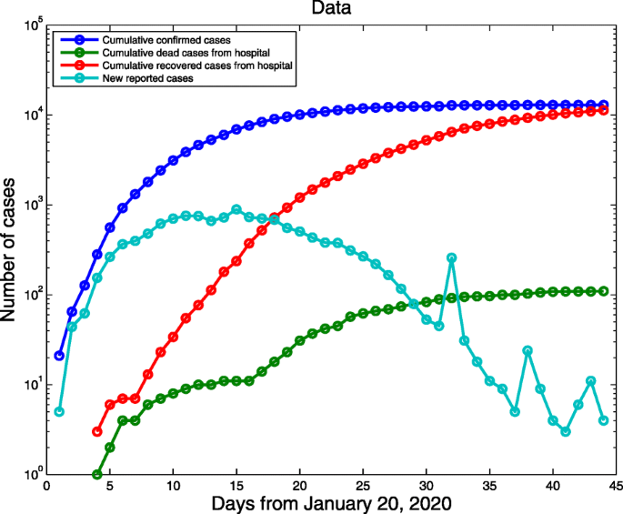
Reported data of the mainland of China excluding Hubei
Parameter estimation
We used the Markov Chain Monte Carlo (MCMC) method with an adaptive Metropolis-Hastings (M-H) algorithm to fit the model. The M-H algorithm, a powerful Markov chain method to simulate multivariate distributions, was executed by using the MCMC toolbox introduced in reference [23]. This toolbox provides tools to generate and analyze Metropolis-Hastings MCMC chains using multivariate Gaussian proposal distribution. The covariance matrix of the proposal distribution can be adapted during the simulation according to adaptive schemes described in references of [24–26].
The algorithm is run for 110 000 iterations with a burn-in of the first 80 000 iterations, and the Geweke convergence diagnostic method is employed to assess the convergence of chains. At the significance level of 5% (the critical value of z is 1.96), all parameters and initial values estimated do not reject the original hypothesis of convergence to a posterior distribution (Fig. 3).
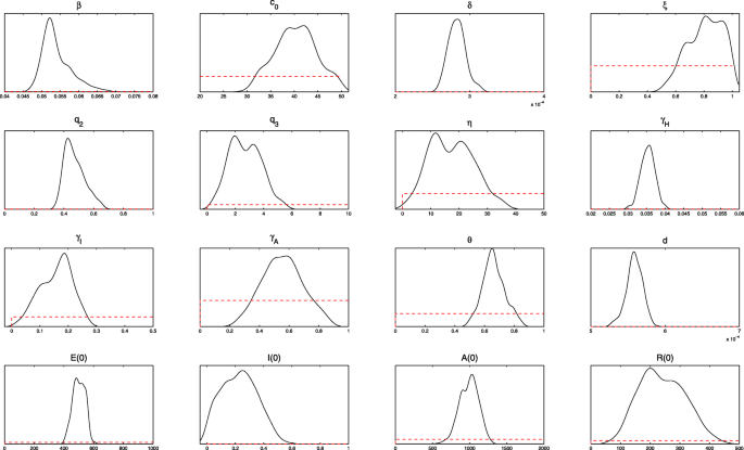
Posterior distribution (solid line) and prior distribution (dash line) of each parameter. x-axis is the parameter value, y-axis is the density
Simulations
The population of the mainland of China excluding Hubei province is around 1 336 210 000 [27], which can be set to be the value of S(0). 21 confirmed cases were reported on 20 January 2020 for the first time and the numbers of recovered and dead individuals were both 0. It can be assumed that nobody has been traced at the beginning. Therefore, we set Si(0)=Q(0)=Rh(0)=D(0)=0, and H(0)=T(0)=21. The quarantined susceptible individuals were isolated for 14 days, thus μ=1/14 [2]. According to reference [7], the incubation period of COVID-19 is about 5.2 days, thus ϕ can be set to be 1/5.2.